Transforms an input sf object into an image overlay for the current height map.
generate_polygon_overlay(
  geometry,
  extent,
  heightmap = NULL,
  width = NA,
  height = NA,
  resolution_multiply = 1,
  offset = c(0, 0),
  data_column_fill = NULL,
  linecolor = "black",
  palette = "white",
  linewidth = 1
)
Arguments
- geometry
An
sfobject with POLYGON geometry.- extent
Either an object representing the spatial extent of the scene (either from the
raster,terra,sf, orsppackages), a length-4 numeric vector specifyingc("xmin", "xmax","ymin","ymax"), or the spatial object (from the previously aforementioned packages) which will be automatically converted to an extent object.- heightmap
Default
NULL. The original height map. Pass this in to extract the dimensions of the resulting overlay automatically.- width
Default
NA. Width of the resulting overlay. Default the same dimensions as height map.- height
Default
NA. Width of the resulting overlay. Default the same dimensions as height map.- resolution_multiply
Default
1. If passing inheightmapinstead of width/height, amount to increase the resolution of the overlay, which should make lines/polygons/text finer. Should be combined withadd_overlay()withrescale_original = TRUEto ensure those added details are captured in the final map.- offset
Default
c(0,0). Horizontal and vertical offset to apply to the polygon, in units ofgeometry.- data_column_fill
Default
NULL. The column to map the polygon fill color to.- linecolor
Default
black. Color of the lines.- palette
Default
black. Single color, named vector color palette, or palette function. If this is a named vector anddata_column_fillis notNULL, it will map the colors in the vector to the names. Ifdata_column_fillis a numeric column, this will give a continuous mapping.- linewidth
Default
1. Line width.
Value
Image overlay representing the input polygon data.
Examples
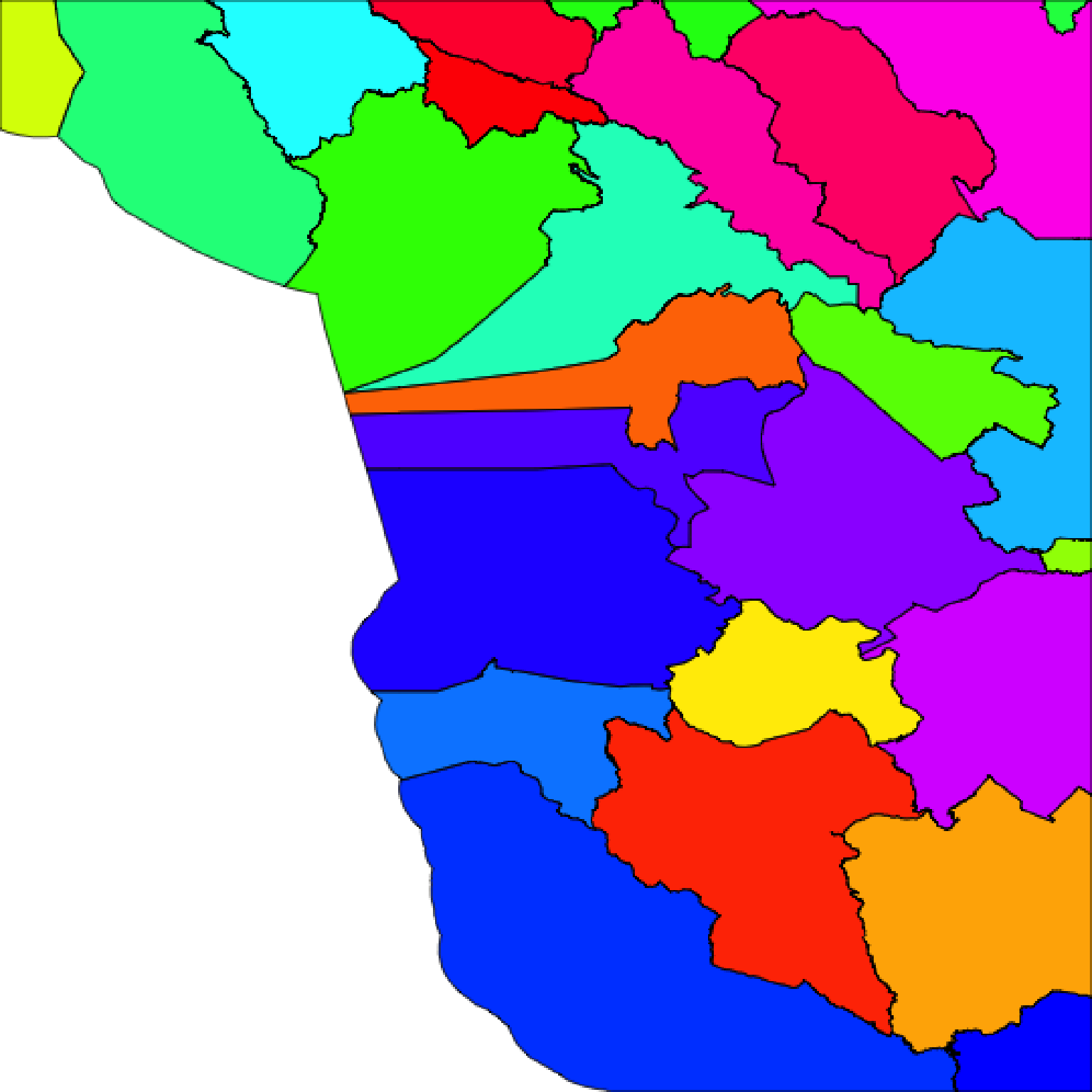
#Plot the counties around Monterey Bay, CA
if(run_documentation()) {
generate_polygon_overlay(monterey_counties_sf, palette = rainbow,
extent = attr(montereybay,"extent"), heightmap = montereybay) |>
plot_map()
}
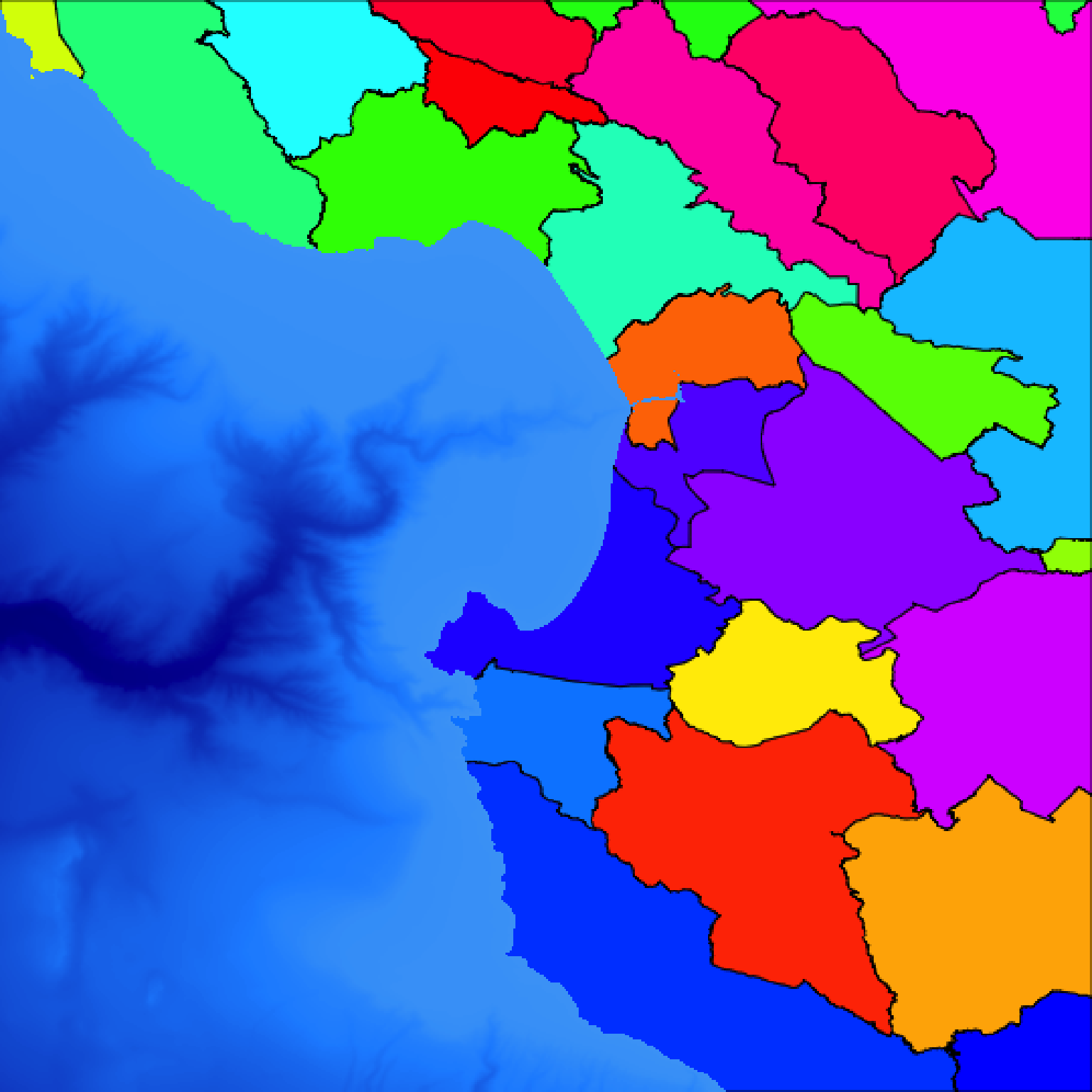
 if(run_documentation()) {
#These counties include the water, so we'll plot bathymetry data over the polygon
#data to only include parts of the polygon that fall on land.
water_palette = colorRampPalette(c("darkblue", "dodgerblue", "lightblue"))(200)
bathy_hs = height_shade(montereybay, texture = water_palette)
generate_polygon_overlay(monterey_counties_sf, palette = rainbow,
extent = attr(montereybay,"extent"), heightmap = montereybay) |>
add_overlay(generate_altitude_overlay(bathy_hs, montereybay, start_transition = 0)) |>
plot_map()
}
if(run_documentation()) {
#These counties include the water, so we'll plot bathymetry data over the polygon
#data to only include parts of the polygon that fall on land.
water_palette = colorRampPalette(c("darkblue", "dodgerblue", "lightblue"))(200)
bathy_hs = height_shade(montereybay, texture = water_palette)
generate_polygon_overlay(monterey_counties_sf, palette = rainbow,
extent = attr(montereybay,"extent"), heightmap = montereybay) |>
add_overlay(generate_altitude_overlay(bathy_hs, montereybay, start_transition = 0)) |>
plot_map()
}
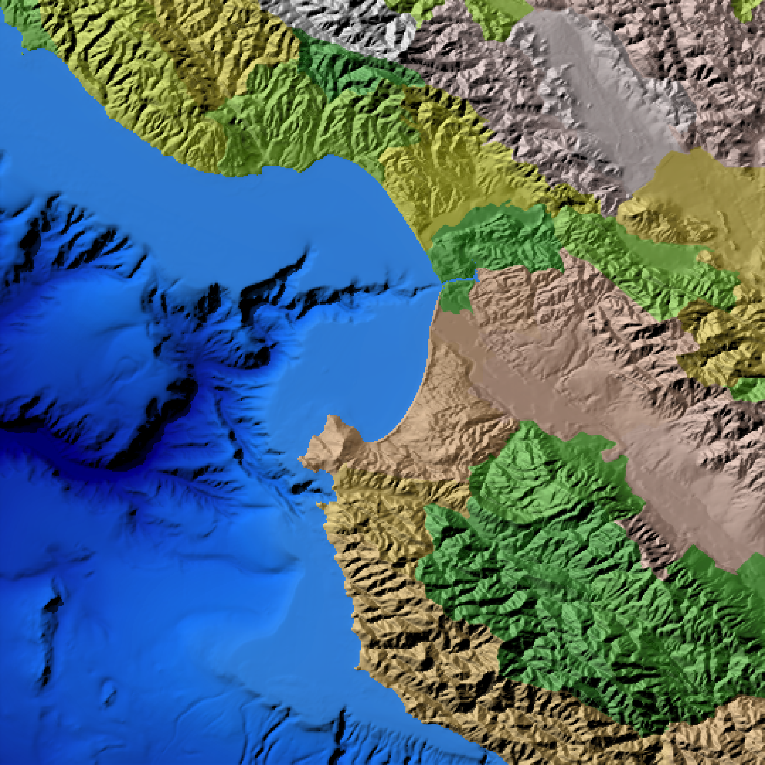
 if(run_documentation()) {
#Add a semi-transparent hillshade and change the palette, and remove the polygon lines
montereybay |>
sphere_shade(texture = "bw") |>
add_overlay(generate_polygon_overlay(monterey_counties_sf,
palette = terrain.colors, linewidth=NA,
extent = attr(montereybay,"extent"), heightmap = montereybay),
alphalayer=0.7) |>
add_overlay(generate_altitude_overlay(bathy_hs, montereybay, start_transition = 0)) |>
add_shadow(ray_shade(montereybay,zscale=50),0) |>
plot_map()
}
if(run_documentation()) {
#Add a semi-transparent hillshade and change the palette, and remove the polygon lines
montereybay |>
sphere_shade(texture = "bw") |>
add_overlay(generate_polygon_overlay(monterey_counties_sf,
palette = terrain.colors, linewidth=NA,
extent = attr(montereybay,"extent"), heightmap = montereybay),
alphalayer=0.7) |>
add_overlay(generate_altitude_overlay(bathy_hs, montereybay, start_transition = 0)) |>
add_shadow(ray_shade(montereybay,zscale=50),0) |>
plot_map()
}
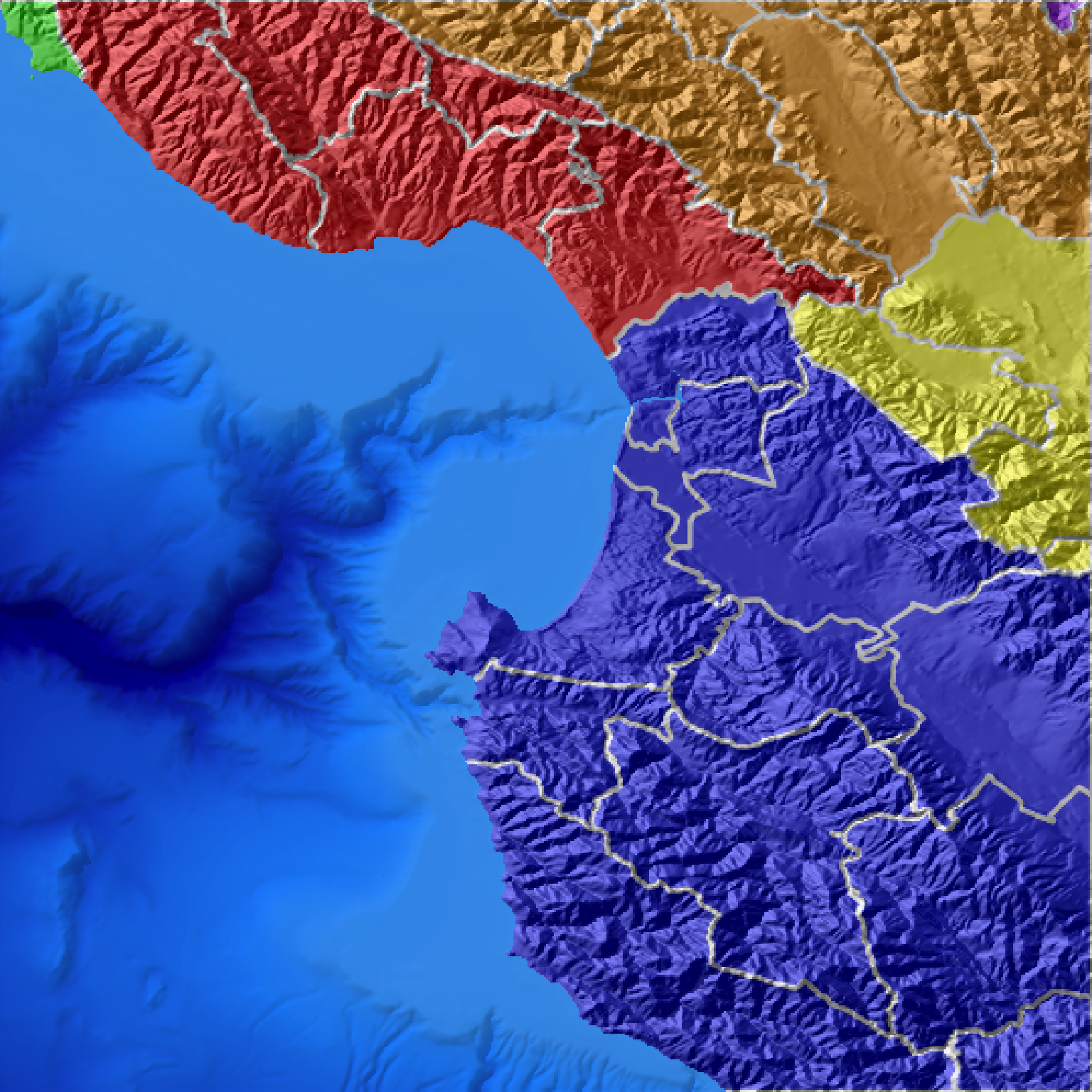
 if(run_documentation()) {
#Map one of the variables in the sf object and use an explicitly defined color palette
county_palette = c("087" = "red", "053" = "blue", "081" = "green",
"069" = "yellow", "085" = "orange", "099" = "purple")
montereybay |>
sphere_shade(texture = "bw") |>
add_shadow(ray_shade(montereybay,zscale=50),0) |>
add_overlay(generate_polygon_overlay(monterey_counties_sf, linecolor="white", linewidth=3,
palette = county_palette, data_column_fill = "COUNTYFP",
extent = attr(montereybay,"extent"), heightmap = montereybay),
alphalayer=0.7) |>
add_overlay(generate_altitude_overlay(bathy_hs, montereybay, start_transition = 0)) |>
add_shadow(ray_shade(montereybay,zscale=50),0.5) |>
plot_map()
}
if(run_documentation()) {
#Map one of the variables in the sf object and use an explicitly defined color palette
county_palette = c("087" = "red", "053" = "blue", "081" = "green",
"069" = "yellow", "085" = "orange", "099" = "purple")
montereybay |>
sphere_shade(texture = "bw") |>
add_shadow(ray_shade(montereybay,zscale=50),0) |>
add_overlay(generate_polygon_overlay(monterey_counties_sf, linecolor="white", linewidth=3,
palette = county_palette, data_column_fill = "COUNTYFP",
extent = attr(montereybay,"extent"), heightmap = montereybay),
alphalayer=0.7) |>
add_overlay(generate_altitude_overlay(bathy_hs, montereybay, start_transition = 0)) |>
add_shadow(ray_shade(montereybay,zscale=50),0.5) |>
plot_map()
}