Plot Map

Displays the map in the current device.

plot_map(
  hillshade,
  rotate = 0,
  asp = 1,
  title_text = NA,
  title_offset = c(20, 20),
  title_color = "black",
  title_size = 30,
  title_font = "sans",
  title_style = "normal",
  title_bar_color = NA,
  title_bar_alpha = 0.5,
  title_just = "left",
  ...
)

Arguments

hillshade

Hillshade to be plotted.

rotate

Default 0. Rotates the output. Possible values: 0, 90, 180, 270.

asp

Default 1. Aspect ratio of the resulting plot. Use asp = 1/cospi(mean_latitude/180) to rescale lat/long at higher latitudes to the correct the aspect ratio.

title_text

Default NULL. Text. Adds a title to the image, using magick::image_annotate().

title_offset

Default c(20,20). Distance from the top-left (default, gravity direction in image_annotate) corner to offset the title.

title_color

Default black. Font color.

title_size

Default 30. Font size in pixels.

title_font

Default sans. String with font family such as "sans", "mono", "serif", "Times", "Helvetica", "Trebuchet", "Georgia", "Palatino" or "Comic Sans".

title_style

Default normal. Font style (e.g. italic).

title_bar_color

Default NA. If a color, this will create a colored bar under the title.

title_bar_alpha

Default 0.5. Transparency of the title bar.

title_just

Default left. Justification of the title.

...

Additional arguments to pass to the raster::plotRGB function that displays the map.

Examples

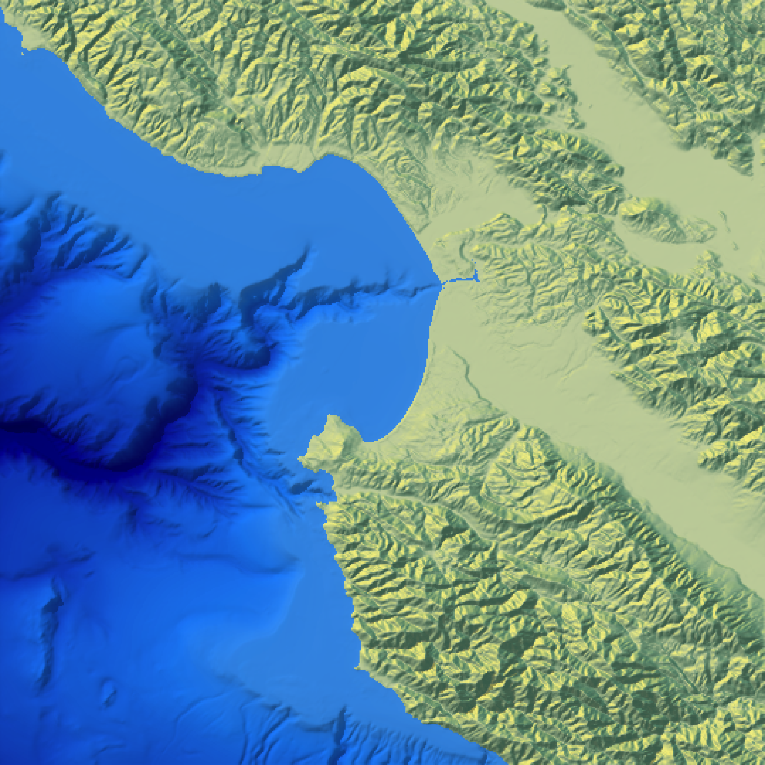
#Plotting the Monterey Bay dataset with bathymetry data
if(run_documentation()) {
water_palette = colorRampPalette(c("darkblue", "dodgerblue", "lightblue"))(200)
bathy_hs = height_shade(montereybay, texture = water_palette)
#For compass text
par(family = "Arial")

#Set everything below 0m to water palette
montereybay %>%
 sphere_shade(zscale=10) %>%
 add_overlay(generate_altitude_overlay(bathy_hs, montereybay, 0, 0))  %>%
 add_shadow(ray_shade(montereybay,zscale=50),0.3) %>%
 plot_map()
}

#Correcting the aspect ratio for the latitude of Monterey Bay

extent_mb = attr(montereybay,"extent")
mean_latitude = mean(c(extent_mb@ymax,extent_mb@ymin))
if(run_documentation()) {
montereybay %>%
 sphere_shade(zscale=10) %>%
 add_overlay(generate_altitude_overlay(bathy_hs, montereybay, 0, 0))  %>%
 add_shadow(ray_shade(montereybay,zscale=50),0.3) %>%
 plot_map(asp = 1/cospi(mean_latitude/180))
}